Papers Explained 335: Transformers without Normalization

This work demonstrates that Transformers without normalization can achieve the same or better performance using a remarkably simple technique. Dynamic Tanh (DyT), an element-wise operation DyT(x) = tanh(αx), is introduced as a drop-in replacement for normalization layers in Transformers. DyT is inspired by the observation that layer normalization in Transformers often produces tanh-like, S-shaped input-output mappings.
Background: Normalization Layers
Most normalization layers share a common formulation. Given an input x with shape (B,T,C), where B is the batch size, T is the number of tokens, and C is the embedding dimension per token, the output is generally computed as:

where ε is a small constant, and γ and β are learnable vector parameters of shape (C, ). They are “scaling” and “shifting” affine parameters that allow the output to be in any range. The terms μ and σ2 denote the mean and variance of the input.
The primary difference between various normalization methods lies in how they calculate the mean (µ) and variance (σ²). This difference affects the dimensions of µ and σ² and how broadcasting is applied during computation.
Batch Normalization (BN): Primarily used in CNNs. Computes mean and variance across both the batch (B) and token (T) dimensions. Formula for mean (µk) and variance (σ²k): µk= (1/BT) * Σi,j xijk and σ²k = (1/BT) * Σi,j (xijk — µk)² Played a significant role in the advancement of deep learning architectures. Other Normalization Layers in CNNs:
Group Normalization: Computes statistics over groups of channels. Instance Normalization: Computes statistics for each channel of each sample independently. Used in tasks like object detection and image stylization.
Layer Normalization (LN): Widely used in Transformer architectures. Computes mean and variance independently for each token in each sample. Formula for mean (µij) and variance (σ²ij): µij = (1/C) * Σk xijk and σ²ij = (1/C) * Σk (xijk — µij)² Favored for its simplicity and general applicability.
Root Mean Square Normalization (RMSNorm): Gaining popularity in large language models (LLaMA, Mistral, Qwen, InternLM, DeepSeek). Simplifies LN by removing the mean-centering step (µij = 0). Formula for variance: σ²ij = (1/C) * Σk x²ijk Normalizes the input using only the root mean square.
What Do Normalization Layers Do
The behaviors of normalization layers in trained networks are empirically studied. For this analysis, a Vision Transformer model (ViT-B) trained on ImageNet-1K, a wav2vec 2.0 Large Transformer model trained on LibriSpeech, and a Diffusion Transformer (DiT-XL) trained on ImageNet-1K are taken. In all cases, LN is applied in every Transformer block and before the final linear projection.

For all three trained networks, a mini-batch of samples is sampled and a forward pass through the network is done. The input and output for the normalization layers are then measured, i.e., tensors immediately before and after the normalization operation, before the learnable affine transformation. Since LN preserves the dimensions of the input tensor, a one-to-one correspondence between the input and output tensor elements can be established, allowing for a direct visualization of their relationship.
For all three models, in earlier LN layers, this input-output relationship is mostly linear, resembling a straight line in an x-y plot. A striking observation from the deeper layers is that most of the curves’ shapes highly resemble full or partial S-shaped curves represented by a tanh function.
For an S-shaped curve, the central part, represented by points with x values close to zero, is still mainly in a linear shape. Most points (∼99%) fall in this linear range. However, there are still many points that clearly fall out of this range, which are considered to have “extreme” values, e.g., those with x larger than 50 or smaller than -50 in the ViT model. Normalization layers’ main effect for these values is to squash them into less extreme values, more in line with the majority of points. This is where normalization layers could not be approximated by a simple affine transformation layer. The non-linear and disproportional squashing effect on extreme values is what makes normalization layers important and indispensable.
Dynamic Tanh (DyT)
Inspired by the similarity between the shapes of normalization layers and a scaled tanh function, Dynamic Tanh (DyT) is proposed as a drop-in replacement for normalization layers. Given an input tensor x, a DyT layer is defined as follows:

where α is a learnable scalar parameter that allows scaling the input differently based on its range, accounting for varying x scales. This is also why the whole operation is named “Dynamic” Tanh. γ and β are learnable, per-channel vector parameters, the same as those used in all normalization layers — they allow the output to scale back to any scales.
Although DyT may look like or be considered an activation function, this study only uses it to replace normalization layers without altering any parts of the activation functions in the original architectures, such as GELU or ReLU.
Experiments
Supervised learning in vision
Vision Transformer (ViT) and ConvNeXt of “Base” and “Large” sizes are trained on the ImageNet-1K classification task.

- DyT performs slightly better than LN across both architectures and model sizes.
Self-supervised learning in vision
Masked autoencoders (MAE) and DINO are benchmarked. Both by default use Vision Transformers as backbones, but have different training objectives: MAE is trained with a reconstruction loss, and DINO uses a joint-embedding loss. Models are first pretrained on ImageNet-1K without using any labels and then tested by attaching a classification layer and fine-tuning them with labels.

- DyT consistently performs on par with LN in self-supervised learning tasks.
Diffusion models
Three Diffusion Transformer (DiT) models of sizes B, L and XL are trained on ImageNet-1K. The patch size is 4, 4, and 2, respectively. In DiT, the LN layers’ affine parameters are used for class conditioning and this is maintained in DyT experiments, only replacing the normalizing transformation with the tanh(αx) function. After training, the Fréchet Inception Distance (FID) scores are evaluated using the standard ImageNet “reference batch”.

- DyT achieves comparable or improved FID over LN.
Large Language Models
LLaMA 7B, 13B, 34B, and 70B models are pretrained to assess DyT performance relative to RMSNorm, the default normalization layer used in LLaMA. The models are trained on The Pile dataset with 200B tokens, following the original recipe. On LLaMA with DyT, a learnable scalar parameter is added after the initial embedding layer, and the initial value of α is adjusted. The loss value after training is reported and the models are benchmarked on 15 zero-shot tasks from lm-eval.

- DyT performs on par with RMSNorm across all four model sizes.
Self-supervised learning in speech
Two wav2vec 2.0 Transformer models are pretrained on the LibriSpeech dataset. The final validation loss is reported.

- DyT performs comparably to LN in both model sizes.
DNA sequence modeling
On the long-range DNA sequence modeling task, the HyenaDNA model and the Caduceus model are pre trained using the human reference genome data from Genome assembly GRCh38.p13. The evaluation is on GenomicBenchmarks.

- DyT maintains performance comparable to LN for this task.
Initialization of α
Initialization of α for Non-LLM Models
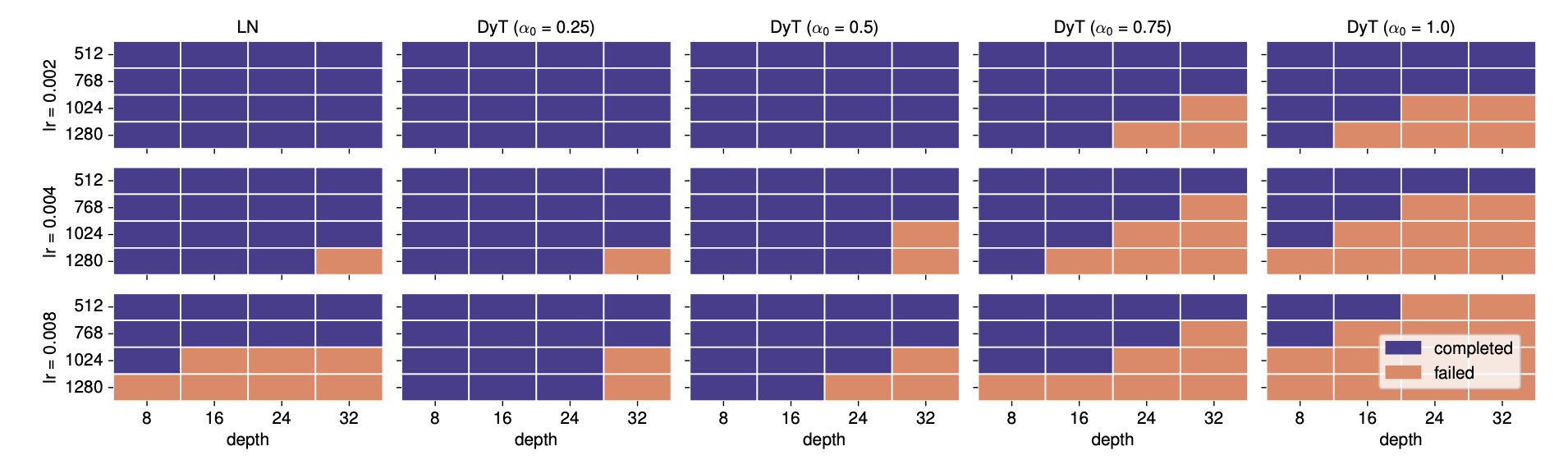
- Insensitivity to α₀: Non-LLM models demonstrate minimal sensitivity to the initial value of α (α₀). A range of α₀ values between 0.5 and 1.2 generally yields good performance, primarily affecting the early stages of training.
- Instability with Larger Values: In certain cases, like supervised Vision Transformer Large (ViT-L) training, higher α₀ values (above 0.6) can lead to training instability and divergence. Reducing the learning rate can mitigate this instability.
- Factors Influencing Stability:
- Larger model sizes require lower α₀ values for stable training.
- Higher learning rates necessitate lower α₀ values for stable training. Conversely, higher α₀ values require lower learning rates.
- Layer Normalization (LN) models exhibit similar stability patterns to DyT with α₀ = 0.5.
- Default Value: Based on these observations, α₀ = 0.5 is recommended as the default for non-LLM models, offering stability comparable to LN while maintaining performance.
Initialization of α for LLMs
- Performance Impact: Tuning α₀ significantly impacts LLM performance, unlike in non-LLM models.
- Key Findings from LLaMA Experiments:
- Larger Models, Smaller α₀: Larger LLMs require smaller α₀ values. The optimal α₀ for smaller models helps narrow the search space for larger models.
- Higher α₀ for Attention Blocks: Initializing α with higher values for DyT layers within attention blocks and lower values for DyT layers in other locations (FFN blocks or before the final linear projection) improves performance. This suggests a nuanced initialization strategy is beneficial.

- Optimal α₀ for LLaMA Models: The table summarizes optimal α₀ values for different LLaMA models, demonstrating the trend of smaller α₀ for larger models and the distinction between attention and other blocks. For instance, a LLaMA 7B model uses 0.8/0.2 while a 70B model uses 0.2/0.05 (attention/other).

- Model Width as Primary Determinant: Model width significantly influences the optimal α₀. Wider models require smaller α₀ values. Model depth has minimal impact. The table illustrates this relationship, showing optimal α₀ values across various widths and depths. Wider networks also require more uneven initialization between “attention” and “other” blocks.
- Hypothesis: The sensitivity of LLMs to α₀ initialization is likely due to their significantly larger widths compared to other models. The wider the model, the more pronounced the need for uneven initialization between attention and other blocks becomes.
Paper
Transformers without Normalization 2503.10622
Hungry for more insights?
Don’t miss out on exploring other fascinating threads in this series. Simply click here and uncover the state-of-the-art research!
Do Subscribe for weekly updates!!