Papers Explained 122: Sparse Transformer

Sparse Transformers introduce sparse factorizations of the attention matrix to reduce the time and memory consumption to O(n√ n) in terms of sequence lengths. It also introduces:
- A restructured residual block and weight initialization to improve training of very deep networks.
- A set of sparse attention kernels which efficiently compute subsets of the attention matrix.
- Recomputation of attention weights during the backwards pass to reduce memory usage.
The same architecture is further used to model images, audio, and text from raw bytes.
Factorized Self-Attention
Qualitative assessment of learned attention patterns
First a qualitative assessment of attention patterns learned by a standard Transformer is performed on an image dataset.

Visual inspection showed that most layers had sparse attention patterns across most data points, suggesting that some form of sparsity could be introduced without significantly affecting performance.
Several layers clearly exhibited global patterns, however, and others exhibited data-dependent sparsity, both of which would be impacted by introducing a predetermined sparsity pattern into all of the attention matrices.
The investigation is thus restricted to a class of sparse attention patterns that have connectivity between all positions over several steps of attention.
Factorized self-attention
A self-attention layer maps a matrix of input embeddings X to an output matrix and is parameterized by a connectivity pattern S = {S1, …, Sn}, where Si denotes the set of indices of the input vectors to which the ith output vector attends. The output vector is a weighted sum of transformations of the input vectors:

Full self-attention for autoregressive models defines Si = {j : j ≤ i}, allowing every element to attend to all previous positions and its own position.
Factorized self-attention instead has p separate attention heads, where the mth head defines a subset of the indices A (m) i ⊂ {j : j ≤ i}. where |A (m) i | ∝ p√ n.
Two-dimensional factorized attention
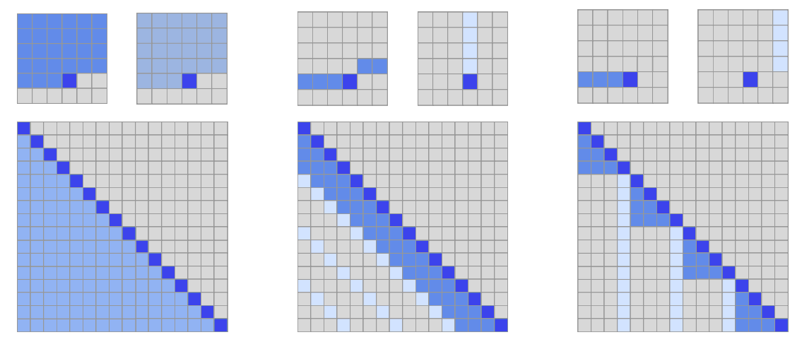
A natural approach to defining a factorized attention pattern in two dimensions is to have one head attend to the previous l locations, and the other head attend to every lth location, where l is the stride and chosen to be close to √ n, this method is called strided attention.
Formally, A (1) i = {t, t + 1, …, i} for t = max(0, i − l) and A (2) i = {j : (i − j) mod l = 0}.
This formulation is convenient if the data naturally has a structure that aligns with the stride, like images or some types of music. For data without a periodic structure, like text, the network can fail to properly route information with the strided pattern, as spatial coordinates for an element do not necessarily correlate with the positions where the element may be most relevant in the future.
In those cases, a fixed attention pattern is used, where specific cells summarize previous locations and propagate that information to all future cells.
Formally, A (1) i = {j : ([j/l] = [i/l])}, where [.] denote the floor operation, and A (2) i = {j : j mod l ∈ {t, t + 1, …, l}, where t = l − c and c is a hyperparameter.
Choosing c ∈ {8, 16, 32} for typical values of l ∈ {128, 256} perform well, although it should be noted that this increases the computational cost of this method by c in comparison to the strided attention.
When using multiple heads, having them attend to distinct subblocks of length c within the block of size l was preferable to having them attend to the same subblock.
Sparse Transformer
The Sparse Transformer is a modified version of the Standard Transformer.
Factorized attention heads
Standard dense attention simply performs a linear transformation of the attend function:
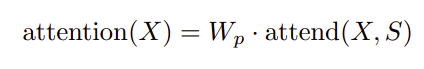
where Wp denotes the post-attention weight matrix. The simplest technique for integrating factorized self-attention is to use one attention type per residual block, and interleave them sequentially or at a ratio determined as a hyperparameter:
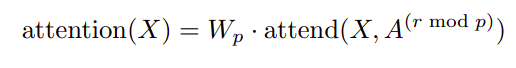
Here r is the index of the current residual block and p is the number of factorized attention heads.
A second approach is to have a single head attend to the locations of the pixels that both factorized heads would attend to, which is called a merged head:
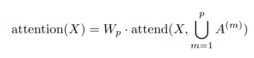
This is slightly more computationally intensive, but only by a constant factor. A third approach is to use multi-head attention, where nh attention products are computed in parallel, then concatenated along the feature dimension:
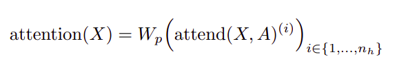
Here, the A can be the separate attention patterns, the merged patterns, or interleaved. Also, the dimensions of the weight matrices inside the attend function are reduced by a factor of 1/nh, such that the number of parameters are invariant across values of nh.
Typically multiple heads work well, though for extremely long sequences where the attention dominates the computation time, it is more worthwhile to perform them one at a time and sequentially.
Scaling to hundreds of layers
Pre-activation residual block are used, defining a network of N layers:
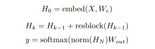
where, Wout is a weight matrix, and resblock(h) normalizes the input to the attention block and a positionwise feedforward network:
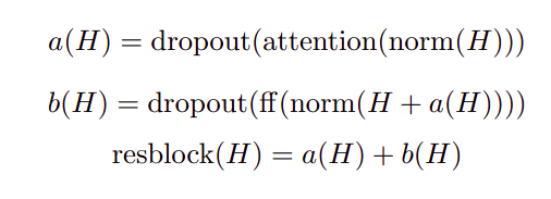
The norm function denotes Layer Normalization, and ff(x) = W2 f(W1x + b1) + b2. f is the Gaussian Error Linear Unit, f(X) = X sigmoid(1.702 · X). The output dimension of W1 is 4.0 times the input dimension.
HN is the sum of N applications of functions a and b, and thus each function block receives a gradient directly from the output layer . The initialization of W2 and Wp are scaled by by 1 /√(2N) to keep the ratio of input embedding scale to residual block scale invariant across values of N.
Modeling diverse data types
Using learned embeddings which either encoded the structure of the data or the factorized attention patterns are important for performance of the models. Hence either n_emb = d_data (number of dimensions of the data) or n_emb = d_attn (number of dimensions of the factorized attention) embeddings are added to each input location.
For images, data embeddings are used, where d_data = 3 for the row, column, and channel location of each input byte. For text and audio, two-dimensional attention embeddings are used, where d_attn = 2 and the index corresponds to each position’s row and column index in a matrix of width equal to the stride.
Saving memory by recomputing attention weights
Gradient checkpointing has been shown to be effective in reducing the memory requirements of training deep neural networks. This technique is particularly effective for self-attention layers when long sequences are processed, as memory usage is high for these layers relative to the cost of computing them.
Through the use of recomputation alone, dense attention networks with hundreds of layers can be trained on sequence lengths of 16,384. In the experiments, the attention and feedforward blocks are recomputed during the backwards pass. To futher simplify the implementation, dropout is not applied within the attention blocks, and instead, it is only applied at the end of each residual addition.
Efficient block-sparse attention kernels
The sparse attention masks can be efficiently computed by slicing out sub-blocks from the query, key, and value matrices and computing the product in blocks.
Attention over a local window can be computed as-is, whereas attention with a stride of k can be computed by transposing the matrix and computing a local window. Fixed attention positions can be aggregated and computed in blocks.
In order to ease experimentation, a set of GPU kernels are implemented which efficiently perform these operations. The softmax operation is fused into a single kernel and also uses registers to eliminate loading the input data more than once, allowing it to run at the same speed as a simple nonlinearity.
The upper triangle of the attention matrix is never computed, moreover, removing the need for the negative bias term of the standard transformer and halving the number of operations to be performed.
Mixed-precision training
Network weights are stored in single-precision floating-point, while network activations and gradients are computed in half-precision. Dynamic loss scaling is used during the gradient calculation to reduce numerical underflow, and half-precision gradients are communicated when averaging across multiple GPUs.
Parameter Initialization
The token embedding We is initialized from N (0, 0.125/√d ) and the position embeddings from N (0, 0.125 √dnemb ).
Within the attention and feedforward components, all biases are initialized to 0 and all weights are initialized from N (0, 0.125 √din ) where din is the fan-in dimension.
The weight matrix for the output logits was initialized to 0.
Experiments
The architectures are empirically tested on density modeling tasks including natural images, text, and raw audio.
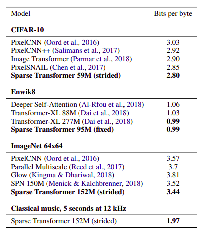
In addition to running significantly faster than full attention, sparse patterns also converged to lower error:
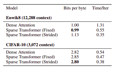
This may point to a useful inductive bias from the sparsity patterns introduced, or an underlying optimization issue with full attention.
Paper
Generating Long Sequences with Sparse Transformers 1904.10509
Hungry for more insights?
Don’t miss out on exploring other fascinating threads in this series. Simply click here and uncover the state-of-the-art research!
Do Subscribe for weekly updates!!